1 Introduction to the comparative method
Rob P. Freckleton
The comparative method is one of the oldest and most widely used approaches in biology [1]. Despite this, the approach may initially be unfamiliar to many because it is frequently not taught as one of the main approaches in research. As we will see in the rest of this book, the comparative method encompasses a family of powerful techniques that can be used to test a wide range of theories, and has applications across the biological sciences.
It is useful to think of there being three ways to address scientific questions: experimental, theoretical or observational [2]. Sometimes described as the ‘gold standard’ [3], experiments test hypotheses by manipulating a small number of factors, whilst other possibly confounding ones are controlled through careful experimental design. This approach has the great advantage that we can be sure that the treatments being varied are definitely the ones that are having an effect on what we measure because the experiment has factored out all unwanted variation. The downsides of experiments are that they can usually only manipulate a small number of factors, they are expensive, and are likely time consuming. For some systems, they may not even be practical: for example we can’t manipulate a whole ecosystem, or we can’t go back in time to do experiments on species that don’t exist any more.
Theory uses mathematical or computer models to create representations of reality. As in a computer game, we can interact with the model to observe the outcomes as we change different parameters. We can undertake virtual experiments, by systematically changing the variables that we are interested in. Models and theory are faster and potentially cheap: a mathematician needs only a pencil, paper and an eraser (a really good one doesn’t even need the eraser…), and the power of modern computers means that we can perform complex simulations that mimic the real world in great detail. However, theory is dependent on our understanding of the system: if we don’t know how a system works, or if we can’t accurately measure the parameters that drive it, then we can’t create a model. In fact, a theory is actually a hypothesis that, at some point, needs to be confronted with hard data.
Observational methods rely on collecting data without changing the system being studied. In some areas of science this is the only possible approach. For example, astronomy is almost entirely dependent on observation as the mechanism for collecting data, because most objects of study are so remote. Similarly, palaeontology is reliant on observations taken of fossils because the study organisms are long dead. Observational methods are potentially extremely powerful, because they are based on data taken directly from natural systems. However, there are pitfalls because they don’t directly account for possible confounding variables in the same way as experiments do, and because it is often not possible to change the system (e.g. astronomy only became an experimental science following the invention of the Death Star).
The Comparative Method is an observational method. It relies on observations and data taken from multiple species in order to test theories. The idea is that a group of species contains more variation than we can observe in a single species, or than we can create in an experiment. Consequently, we can use data on groups of species to test hypotheses using wider range of variation than we could ever generate in a single one. The problem, however, is that whilst factors we are interested in measuring will vary across species, there will also be variation in many other variables and this can lead to considerable problems. This aim of this book is to explain this problem and how we can use clever statistical methods to deal with it. There is now an extensive and potentially confusing literature on comparative methods [4]. The literature on the ‘modern’ comparative method extends over 40 years. Some of the literature is highly technical, including advance mathematics and statistics. At face value it is a daunting prospect to master this body of work and start to use it in practice.
Having said that, the principles that underpin comparative methods are relatively simple to understand. Moreover, despite the plethora of methods, many of them are closely related and linked by similar statistical and evolutionary models. The rationale for our book is that by understanding a few key concepts and methods, it is possible to enter this outwardly daunting field and quickly work on real problems.
1.1 Historical context of the comparative method
As we mentioned above the comparative method is old: arguably the first example of comparisons was by Edward Tyson in 1699 who looked at the similarities and differences between different apes and hominids [5]. Using these comparisons, he was able to demonstrate that there is more similarity between chimpanzees (Pan sp.) and humans (Homo sapiens) than between chimpanzees and humans. Even in the absence of Darwinian evolutionary theory, this work was clearly instrumental in generating the underpinnings of our subsequent understanding of evolutionary relationships. Subsequently, the field of comparative anatomy emerged, which was probably the dominant approach for studying whole organism biology in the 18th and 19th centuries.
The modern era of the comparative method perhaps begins with the pioneering work of Tinbergen. Tinbergen was interested in the eggshell removal behaviour of black-headed gulls (Chroicocephalus ridibundus). Tinbergen hypothesised that removal of eggshells from their ground nests was an adaptive behaviour to reduce predation by other gulls. This hypothesis was supported by observations on black-legged kittiwakes (Rissa tridactyla) which do not remove eggshells because they nest on cliffs, thereby avoiding predators.
Tinbergen’s work was influential and exemplifies comparative ideas in framing and testing hypotheses. However, there are two obvious limitations. First, the study only considers two species and second, the analysis is qualitative. Nowadays comparative studies use observations from many more species. Indeed, it is not unusual to see modern comparative analyses applied to thousands of species: comparative analyses of birds, for example, can now be be conducted on all ~11000 species of birds because of the availability of data and a comprehensive phylogeny for this group. As the comparative method has evolved, studies have progressed from using simple familiar methods such as correlation and regression, through more complex methods such as nested ANOVAs, to the current suite of tests that take advantage of developments at the forefront of statistical science.
This evolution of the methods reflects a recognition of the inherent complexity of datasets, as well as increasingly sophisticated thinking about the way that evolution shapes comparative data. However, the underpinning logic of testing ideas by looking at patterns across different species is very well established.
1.2 What questions can we answer with comparative methods?
What types of question can we answer using comparative approaches? The answer is ‘almost any’! We outline some that we will focus on later in this book below. As we mentioned above, comparative methods are especially useful when it is not possible to perform an experiment. Any group of species will exhibit more variation in life-history, ecology or behaviour that any single species, or that we could artificially create in an experiment. Comparative methods are therefore powerful alternatives that permit us to test extremely broad hypotheses.
Comparative approaches can exploit ‘natural experiments’. Tinbergen’s work on black-headed gulls and kittiwakes is a good example of this. By choosing species that differ in a few key respects, but are similar in others, it is possible to analyse what amounts to an experiment, but using natural variation.
The comparative method is best suited for testing existing hypotheses that have been stated in advance. As we shall see, comparative approaches generate large datasets with many variables. Analysing large complex datasets in the absence of pre-defined hypotheses is fraught with potential dangers and can be prone to data-dredging and p-hacking. For example, if we conduct 20 statistical tests using the conventional threshold of p < 0.05, one test will be statistically significant on average, even if there are no relationships or effects in our dataset. If our dataset contains 20 variables then we could perform as many as 180 pairwise correlations. The null expectation is that these would yield 9 significant results just by chance. Data-dredging is the practice of trawling through datasets looking for such results and presenting them as if these were the hypotheses we sought to test at the outset.
This multiplicity of results is particularly a problem if the process is not described completely. For example, if we report that we have tested 180 correlations and found statistical significance for 9 of them, then the strength of belief in the result would be low. However, if we presented these 9 results without fully explaining that these are the tip of a statistical iceberg, then the impression would be created that the strength of evidence is much stronger. The practice of ‘p-hacking’ is a known problem in such analyses.
Although data-mining approaches may have a place, in most comparative analyses the best approach is to focus on pre-defined theories and hypotheses. That is, a set of hypotheses are proposed, the required data are collected, and statistical tests are performed to test the hypotheses as they were envisaged.
What questions can we answer with PCMs?
This book features many examples of questions we can tackle using phylogenetic comparative methods. We’ve listed these below. We think it is important to highlight diverse contributions to science, so our examples highlight work by a diverse range of authors working in the field today. Check these out in later chapters!
- Chapter 2: Are eye size and ecology related in frogs and toads? Thomas et al. (2020) [6].
- Chapter 3: What was the litter size of the ancestral bat? Garbino et al. (2021) [7].
- Chapter 4: Is there phylogenetic signal in how Rhododendron species respond to climate change? Basnett et al. (2019) [8].
- Chapter 4: Do ticks transmit trypanosomes? Koual et al. (2023) [9].
- Chapter 5: Do rates of body size evolution in mammals with different foot postures? Kubo et al. (2019) [10].
- Chapter 5: What are the ecological mechanisms underpinning the adaptive radiation of Phylloscopus warblers? Price et al. (1997) [11].
1.3 The problem of phylogenetic non-independence
We highlighted above that in experiments we use careful design to control for unwanted confounding variation. This cannot be controlled directly in observational approaches. Consequently there is a danger that observational methods could generate misleading results.
The naive way to perform a comparative analysis would be to collect data across a group of species, conduct a statistical analysis and then interpret the results. In data collected on groups of species, there is a special problem that data are expected to be statistically non-independent because of phylogenetic relationships among the species. As explained below, non-independent data are a problem for conventional statistical methods, and break one of the key assumptions of most statistical tests.
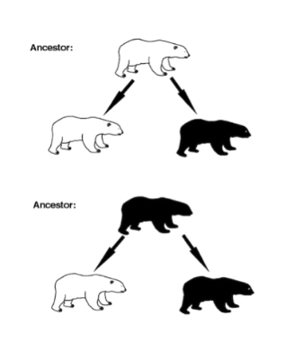
Phylogenetic non-independence is a special case of non-independent data that arises because of the evolutionary relationships between species. Two species that have evolved from a common ancestor share many characteristics because of common ancestry, not because of independent evolution. Figure 1.1 gives a hypothetical example (after [1]).
Imagine that we study two species of bears, white bears and black ones. We might reasonably hypothesise that white colouration is an adaptation to snowy environments and black colouration is an adaptation to dark forest environments. If we find that the white bears are found in snowy conditions and black bears live in forests, we might think that the hypothesis is supported. However, as shown in Figure 1.1 there could be two evolutionary paths by which we arrive at the current state: it could be that the extant species evolved from either a black or a white ancestral parent species. Our belief in the hypothesis then depends on where the ancestor lived. For instance, if the ancestor was white and lived in snowy conditions, or if the ancestor were black and lived in forests, then the hypothesis would still be supported. In the former case, the black coat might have evolved as an adaptation during the move to forests and in the latter case the white coat evolved along with the move to snowy conditions.
However, if the ancestor lived in different conditions then our conclusion may not be so certain. On the assumption that this species was perfectly well adapted to their environment, if it were white and lived in the forest, or were black and lived in snowy conditions, or if both black and white species occur in both environments, we would be less sure that current coat colour was the outcome of selection. It could be that coat colour evolves in response to some other factor that we haven’t measured or considered.
This is an example of the problem of phylogeny in comparative analyses. We cannot assume that current patterns reflect evolutionary processes. The traits that species currently possess are inherited from their ancestors in addition to being shaped by more recent selective pressures. Treating the traits from present-day species as if they had evolved completely independently could lead to misleading conclusions.
How could we overcome the problem in this case? There are a couple of options: if fossil data are available then it might be possible to look at the ancestors and retrace the evolution of coat colour. This is unlikely, however, as the fossil record is usually very patchy and incomplete. Taking a comparative approach, and alternative solution might be to look for further species pairs: e.g. mountain hares, arctic foxes, and stoats have white coats (at least in winter) and these could be contrasted with closely related species that do not. If we see the same pattern repeated across several independent taxa, we may become more confident in the coat-colouration hypothesis. This solution is very much the philosophy of the comparative approach: variation across lots of species allows us to test hypotheses more robustly. The issue of phylogenetic non-independence is dealt with by choosing pairs of species that are similar in most respects (e.g. ecology, life history, diet) except the one we are interested in (coat colour). This is akin to the tactic of ‘blocking’ in experimental design.
\[\\[0.5cm]\]
In this example, we need to understand the distribution of traits in the ancestors, as well as where they lived, in order to robustly test the hypothesis in question. Species inherit traits from ancestors and the traits of ancestors shape the traits of their descendants. The most important lesson from this example is that even in very simple comparative analyses we need to understand the evolutionary relationships among species. This insight applies to any comparative analysis: we cannot regard species as being evolutionarily independent and we have to account for this non-independence when analysing comparative data.
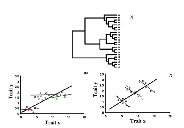
The example shown in Figure 1.1 is very simple and the problem of phylogeny is that it impedes the interpretation of the data. However there can also be statistical problems resulting from phylogenetic non-independence and this becomes apparent when we try to perform more sophisticated statistical analysis. Figure 1.2 shows another hypothetical example to illustrate this. Figure 1.2(a) presents a phylogeny of 21 species. A naive comparative analysis would ignore the relationship represented by this phylogeny and treat all of the species as if they are equal. However, Figures 1.2(b) and (c) show the problem of doing this when we analyse trait data. In both cases, data has been collected on two traits (‘X’ and ‘Y’) for each of the species. This is a very typical comparative analysis, and we would usually use linear regression or correlation to look for evidence of a correlation between the two traits. In both of these figures, the thick bold line is the relationship we obtain by doing this and performing a simple analysis that treats all species as equal, ignoring the evolutionary relationships between them.
\[\\[0.5cm]\]
In both cases the analysis indicates that there is a strong positive relationship between the two traits. However, when we recognise that species are related according to the phylogeny in Figure 1.2(a), it is evident that the situation is more complex. In Figure 1.2(a) we can recognise three distinct clades (coloured separately). Looking at Figure 1.2(b) and (c), it is clear that within any of the clades the relationship between X and Y is very different from the picture we obtain overall. In Figure 1.2(b) the relationships are quite weak, while in Figure 1.2(c) the relationships between X and Y are negative within the clades although positive overall.
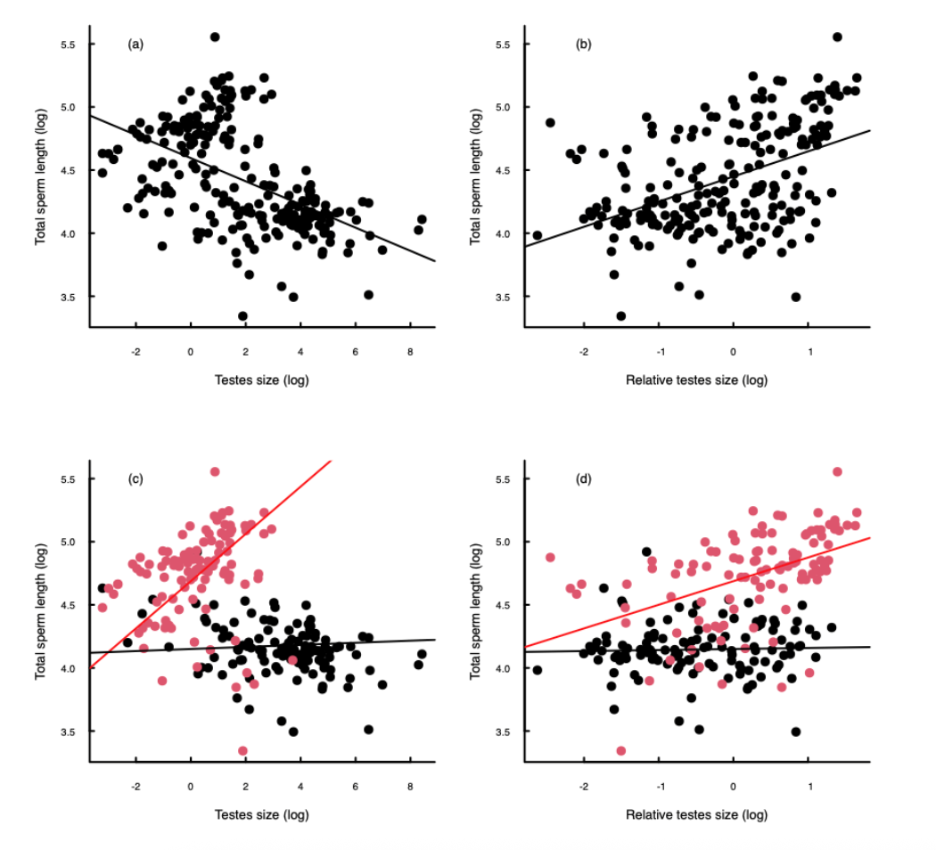
Although Figure 1.2 shows a hypothetical scenario, such patterns can emerge in real data. Figure 1.3 shows some real data in which the phylogenetic structure of the dataset influences the overall conclusion. The data show the relationship between testes size and sperm length in mammals (note that all data have been log transformed). The reason for looking at this relationship was to test hypotheses about sperm competition and sexual selection (we don’t have the space to go into this here).
Figure 1.3(a) and 1.3(b) show the relationships between sperm length and testes size (Figure 1.3(a)) and between sperm length and relative teste size (testes size relative to body mass; Figure 1.3(b)). Linear regression (the solid lines) suggest that there is a strong negative relationship between sperm length and testes size (Figure 1.3(a)) and conversely that there is strong positive relationship between sperm length and relative testes size (Figure 1.3(b)). Although these relationships look reasonably convincing, unfortunately there is a strong influence of phylogeny in the data. In Figures 1.3 (c) and (d) the same data are plotted, but the colours indicate the phylogenetic structure of the data. The red points show data from rodents (order Rodentia), whilst the black points are data from all other mammals. It is very clear that the patterns are very different in the rodents: there is a strong positive correlation between sperm length and testes size in rodents and no relationship in the others mammals (Figure 1.3(c)); similarly there is also a strong positive correlation between sperm length and relative testes size in rodents, but no relationship in the other mammals (Figure 1.3(d)).
\[\\[0.5cm]\]
In this example the problems are several-fold. Clearly the evolution of sperm length with testes size has been very different in the rodents compared with other mammals. If we treat each data point as if it were statistically independent (as in Figure 1.3(a) and (b)), this overlooks this difference and we get an incorrect conclusion.
There is also a more general issue, what is sometimes called the ‘degrees of freedom’ problem. The problem here is, even if the relationship between the two traits were the same for both of these clades we cannot treat the data as being statistically independent, meaning that each point does not contribute an independent degree of freedom to the analysis. Species that are closely related are likely to have similar values of both traits, simply because they share common ancestry. The outcome of this is akin to assuming ‘too many’ degrees of freedom in the analysis: if we have data on 100 species, because of phylogenetic relatedness we probably have less than 100 independent data points. However, conventional statistical analyses assume that the points are independent of each other and this will lead to incorrect statistical outputs and conclusions. This issue has motivated a lot of research on comparative methods over the past 40 years.
1.4 How do comparative methods work?
The problem of phylogeny is that species inherit their traits from their ancestors, meaning that we cannot assume that current patterns of trait variation reflect independent evolution. We need to understand the phylogenetic pattern of trait evolution in order to properly test hypotheses about the current distribution of values. For instance, in Figure 1.1 we need to know by which route coat colour evolved as well as the corresponding habitats in which species lived.
Of course, we typically don’t have any information at all on the traits of the ancestral species. As mentioned above, fossil data are patchy at best so that we can rarely directly trace the evolution of traits from ancestors to descendants. However, we have a phylogeny for many groups of species, which means that we do know how closely or distantly the species are related to each other in an evolutionary sense.
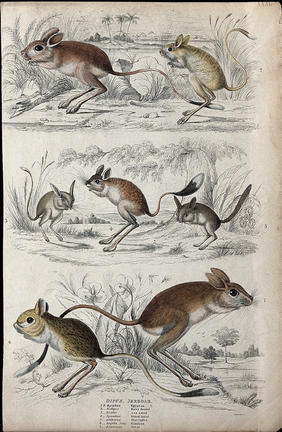
We can reasonably expect that species that are closely related to each other are more similar than to distantly related ones. Figure 1.4 gives an example of this. This plays out across a phylogeny, so that we expect to see a clear imprint of phylogeny in the distribution of trait values, called phylogenetic signal. In Chapter 4 we go into more detail about this. For now, the important thing is this signal can be used to help us to overcome the problem of phylogeny in comparative analyses. The seven species shown in Figure 1.4 are all close relatives that share common ancestry. Given the degree of similarity between them, it would not be hard to make a guess about what the ancestors were like: in all probability they all had brown coats and long back legs for example! But we can go further
\[\\[0.5cm]\]
In the absence of fossil data, we use an evolutionary model to achieve this. A model for trait evolution is a mathematical description of the changes in traits over evolutionary time. Using such a model we can take data on extant species and work backwards through the phylogeny to infer what the traits of the ancestors would have been. The model is essentially a statistical description of the ancestral values that are most likely to have given rise to the current trait values, given specific assumptions about the way that evolution proceeds. This may seem somewhat nebulous at this point, in Chapter 3 we start to flesh this out in more detail.
Effectively, comparative methods work by using this phylogenetic information to fill in the gaps in our knowledge of ancestral trait values. What all comparative methods do, either explicitly or implicitly, is to estimate values for the ancestors in order to map the evolution of traits through the phylogenetic tree. When we look at several traits, we then examine the correlation between the changes in traits across the phylogeny to test whether their evolution is linked.