7 Phylogenetic generalised linear mixed models in R
The aims of this exercise are to learn how to use R to perform Phylogenetic Generalised Linear Mixed models (PGLMM)in R using MCMCglmm.
We will be using the evolution of eye size in frogs as an example. The data and modified tree come from [2], and the original tree comes from [3]. I’ve removed a few species and a few variables to make things a bit more straightforward. If you want to see the full results check out Thomas et al 2020 [2]!
Before you start
Open your R Project. Mine is a folder called PCM-exercises, and it is named PCM-exercises.RProj. Within the PCM-exercises folder is a subfolder called data where I have stored all the data I downloaded from here.
You will also need to install the following packages:
7.1 Why fit phylogenetic generalised linear mixed models?
Up this point we have been working with models where our diagnostic plots look pretty good, and where the residuals are roughly normally distributed. Unfortunately this is not the case for all models, especially those with particular kinds of response variables.
Where response variables are counts (e.g. number of individuals) we don’t expect normally distributed residuals because counts can only be whole numbers, and cannot go below zero. Instead count data are usually pretty well described by a Poisson distribution instead. Where response variables are binary (e.g. 0 or 1) or proportion data, we also don’t expect to see normally distributed residuals because again these variables cannot be negative, and in the case of binary data cannot be anything other than 0 or 1, and in the case of proportion data can only be between 0 and 1. Binary/proportion data are usually pretty well described by a binomial distribution instead. In your statistics classes you may have heard that the solution in these cases is to fit a generalised linear model, glm in R (rather than just a linear model; lm in R). We need to add this generalised linear modelling framework if we want to use count, or proportion, or binary response variables in our models.
Unfortunately, there is not an easy way to extend PGLS to do this, so we need another kind of model. There are a number of ways to incorporate phylogenetic information into statistical methods based on a variety of statistical models. We focus on the PGLS model because it’s quite easy to understand how it works, and uses standard models that we (should be) are already familiar with from basic statistics.
Another way we can incorporate phylogenetic information into a model is by using a mixed effects model. Mixed effects models have fixed effects, usually the variables we are interested in investigating, and random effects, often “nuisance” variables that we might need to control for in our analysis, or information about the hierarchical nature of the model set up. We can add information about the phlyogeny into the random effects componenet of a mixed effects model. Mixed effects models are very useful, but very hard to fully understand.
Luckily, there is a package in R called MCMCglmm that performs generalised linear mixed models (GLMM), i.e. mixed effects models that are generalised to deal with response variables that result in non-normally distributed residuals. This package also allows us to add our phylogenetic information as a random effect in the model. Great!
Unfortunately, fitting these models is quite tricky, in part because of the MCMC part of the MCMCglmm package name. MCMC stands for Markov Chain Monte Carlo, and this is a Bayesian method which means it works somewhat differently to the models we’ve met before. I’ll try to explain as we go along.
Bayesian phylogenetic generalised mixed models are very powerful tools, but can be complicated to understand and difficult to use properly. Before jumping in to these it is vital that you have a good understanding of generalised linear models (GLMs), and generalised linear mixed models (GLMMs) including how to fit and interpret the outputs of these models in R. This is beyond the scope of this book. If you feel uncomfortable with these we suggest you go back and learn these methods first. You also need a basic understanding of Bayesian statistics.
7.2 A really quick reminder of how Bayesian analyses work, with apologies to Bayesian scholars for the simplification!
Bayesian methods calculate the probability of the model given the data, P(model|data), i.e. the reverse of Maximum Likelihood.
To fit Bayesian models we first assign a set of priors. These are our hypotheses about how we think the world works. They provide a starting point for the MCMC algorithm to search model space.
I like to think of Bayesian MCMC algorithms as a little robot friend wandering about. The robot starts where the priors suggest it should, then searches the virtual space of all possible model fits to find the parameters for your model (e.g. slopes and intercepts). The first few (hundreds, thousands, sometimes millions depending on the model!) tend to be poor attempts as the robot is still getting oriented, so we exclude these from the output as burnin. The robot keeps going until it’s tried as many models as you asked for (again this can be thousands to millions depending on the model). Because the robot will find very similar results close together due to the nature of the way it searches, we say that the results are autocorrelated. To deal with this, we only sample the results every so often, rather than sampling all of them. This is called thinning and we tell the robot in advance how we want to thin the sample (usually we ask for an answer every couple of thousand attempts).
Finally the robot gives us a distribution of results (often thousands or even millions), that we call the posterior distribution (or just the posterior). The posterior is a sample of all possible results across all of models fitted, in proportion to their posterior probability. This means there will be a range of results in the posterior, but those the robot encountered more often will appear more often, and those it encountered rarely will appear less often.
Before we look at the results, we need to check that the robot did a good job and converged on a sensible set of results, rather than wandering all over the place like it did during the burnin phase. We generally look at trace plots to assess this (see below) and also calculate Effective Sample Size or ESS. ESS of over 200 suggests the model has converged, and we can then go on to look at our results.
This is a simplification of course! But the take home is that to fit MCMCglmm models we need to consider priors, burnin, number of iterations, thinning, convergence and the posterior. In addition to the model, data and phylogeny that we’ve been considering in previous examples…
If you want to learn more about Bayesian statistics we highly recommend [37] and the accompanying online course.
Now let’s try a practical example…
7.3 Preparation
To begin we need to load the packages for this practical.
Next we need to prepare the tree and data for the analyses. In the Preparation exercise (see 4) we read in our tree and data, checked them, and matched them so only species in both were retained. Please refer to that exercise for more details on how and why we do these things, or run through it now if you haven’t previously. Hopefully you’re pretty comfortable with this by now.
# Read in the data
frogdata <- read_csv("data/frog-eyes.csv")
# Check everything loaded corrected
glimpse(frogdata)
## Rows: 215
## Columns: 11
## $ Binomial <chr> "Allophryne_ruthveni", "Eupsophus_roseus", "Alytes_obstetrican…
## $ Family <chr> "Allophrynidae", "Alsodidae", "Alytidae", "Alytidae", "Aromoba…
## $ Genus <chr> "Allophryne", "Eupsophus", "Alytes", "Discoglossus", "Allobate…
## $ tiplabel <chr> "Allophryne_ruthveni_Allophrynidae", "Eupsophus_roseus_Alsodid…
## $ Adult_habitat <chr> "Scansorial", "Ground-dwelling", "Ground-dwelling", "Ground-dw…
## $ Life_history <chr> "Free-living larvae", "Free-living larvae", "Free-living larva…
## $ Sex_dichromatism <chr> "Absent", "Absent", "Absent", "Absent", "Absent", "Absent", "A…
## $ SVL <dbl> 23.76667, 38.37500, 37.46667, 62.64000, 25.60000, 27.03333, 38…
## $ mass <dbl> 1.0000000, 7.5000000, 6.6666667, 24.4000000, 2.1000000, 2.4666…
## $ rootmass <dbl> 0.9917748, 1.9273451, 1.8690601, 2.8885465, 1.2549697, 1.35076…
## $ eyesize <dbl> 3.200000, 5.362500, 6.366667, 7.550000, 4.116667, 3.783333, 4.…# Read in the tree
frogtree <- read.nexus("data/frog-tree.nex")
# Check it loaded correctly
str(frogtree)## List of 4
## $ edge : int [1:426, 1:2] 215 216 217 218 219 220 221 222 223 224 ...
## $ edge.length: num [1:426] 0.166 0.114 0.102 0.4 0.133 ...
## $ Nnode : int 213
## $ tip.label : chr [1:214] "Ascaphus_truei_Ascaphidae" "Leiopelma_hochstetteri_Leiopelmatidae" "Alytes_obstetricans_Alytidae" "Discoglossus_pictus_Alytidae" ...
## - attr(*, "class")= chr "phylo"
## - attr(*, "order")= chr "cladewise"## [1] TRUE## [1] TRUE## [1] TRUE# Check whether the names match in the data and the tree
check <- name.check(phy = frogtree, data = frogdata,
data.names = frogdata$tiplabel)
# Look at check
check## $tree_not_data
## [1] "Incilius_nebulifer_Bufonidae" "Leptobrachella_bidoupensis_Megophryidae"
## [3] "Microhyla_fissipes_Microhylidae" "Microhyla_marmorata_Microhylidae"
##
## $data_not_tree
## [1] "Gastrophryne_carolinensis_Microhylidae" "Leptobrachella_dringi_Megophryidae"
## [3] "Megophrys_gerti_Megophryidae" "Microhyla_pulverata_Microhylidae"
## [5] "Oreobates_quixensis_Strabomantidae"# Remove species missing from the data
mytree <- drop.tip(frogtree, check$tree_not_data)
# Remove species missing from the tree
matches <- match(frogdata$tiplabel, check$data_not_tree, nomatch = 0)
mydata <- subset(frogdata, matches == 0)
# Look at the tree summary
str(mytree)## List of 4
## $ edge : int [1:418, 1:2] 211 212 213 214 215 216 217 218 219 220 ...
## $ edge.length: num [1:418] 0.166 0.114 0.102 0.4 0.133 ...
## $ Nnode : int 209
## $ tip.label : chr [1:210] "Ascaphus_truei_Ascaphidae" "Leiopelma_hochstetteri_Leiopelmatidae" "Alytes_obstetricans_Alytidae" "Discoglossus_pictus_Alytidae" ...
## - attr(*, "class")= chr "phylo"
## - attr(*, "order")= chr "cladewise"## Rows: 210
## Columns: 11
## $ Binomial <chr> "Allophryne_ruthveni", "Eupsophus_roseus", "Alytes_obstetrican…
## $ Family <chr> "Allophrynidae", "Alsodidae", "Alytidae", "Alytidae", "Aromoba…
## $ Genus <chr> "Allophryne", "Eupsophus", "Alytes", "Discoglossus", "Allobate…
## $ tiplabel <chr> "Allophryne_ruthveni_Allophrynidae", "Eupsophus_roseus_Alsodid…
## $ Adult_habitat <chr> "Scansorial", "Ground-dwelling", "Ground-dwelling", "Ground-dw…
## $ Life_history <chr> "Free-living larvae", "Free-living larvae", "Free-living larva…
## $ Sex_dichromatism <chr> "Absent", "Absent", "Absent", "Absent", "Absent", "Absent", "A…
## $ SVL <dbl> 23.76667, 38.37500, 37.46667, 62.64000, 25.60000, 27.03333, 38…
## $ mass <dbl> 1.0000000, 7.5000000, 6.6666667, 24.4000000, 2.1000000, 2.4666…
## $ rootmass <dbl> 0.9917748, 1.9273451, 1.8690601, 2.8885465, 1.2549697, 1.35076…
## $ eyesize <dbl> 3.200000, 5.362500, 6.366667, 7.550000, 4.116667, 3.783333, 4.…# Convert to a dataframe
mydata <- as.data.frame(mydata)
# Check this is now a data frame
class(mydata)## [1] "data.frame"7.4 MCMCglmm specific preparation
7.4.1 Inverse phylogenetic variance-covariance matrix
For MCMCglmm we need the inverse of the phylogenetic variance-covariance matrix.
To do this, we first need the tree to have no zero-length branches. In 04-Preparation you may recall that we deal with polytomies by replacing them with zero length branches using the ape function multi2di. To remove the zero length branches we are going to use the opposite function: di2multi. This deletes all zero length branches and collapses them back into polytomies.
Although not an issue here, inverseA (see below) can break if your tree has node labels. We can remove these using:
Now we can get the inverse of the phylogenetic variance-covariance matrix using the function inverseA.
# Get the inverse vcv matrix for the phylogeny
inv.phylo <- inverseA(mytree2, nodes = "TIPS", scale = TRUE)$Ainv
nodes = "TIPS" means that we are only including the tips in the calculation. We can use nodes = "ALL" to include ancestral nodes in the calculation. scale = TRUE means the tree is scaled so that total branch length from root to tips, is equal to one. This makes the model a bit easier to fit, but only works with ultrametric trees. For non-ultrametric trees you need to set this as FALSE.
Using nodes = "TIPS" can mean it takes longer for the model to run. Very large phylogenies usually require nodes = "ALL" or MCMCglmm won’t even run.
However, nodes = "ALL" can result in higher auto-correlation (see below).
7.4.2 Priors
MCMCglmm requires us to set prior distributions for the fixed and random effects. For the random effects this is actually a bit trickier than many help tutorials might suggest. If you’re fitting any model with any degree of complexity you’ll need to read up on this to get the most appropriate priors.
The default prior for the fixed effects is a Normal distribution with a mean (mu) of 0 and variance (V) of 1^10. This is known as a diffuse prior, as the variance is so large the prior is basically saying that the fixed effects can be pretty much any number, positive or negative. Generally this is fine so we don’t tend to change this from the default.
For the random effects we need to define a set of priors for the variance components of each random effect. MCMCglmm uses something called an inverse Wishart distribution for the random effects prior, and this is described by two parameters: the variance (V) and degree of belief (nu). This distribution tends to be right-skewed when nu is small.
Often in examples you’ll see people using priors where V = 1 and nu = 0.02. This prior specification is used a lot because it was believed to be relatively uninformative (it is also equivalent to an inverse-gamma prior with shape and scale of 0.001, for anyone more familiar with that distribution). It is generally is fairly uninformative, but can behave inappropriately when the posterior distribution for the variances has support close to zero. In these cases it’s worth looking at the parameter expanded priors section of the MCMCglmm course notes for some solutions.
Using priors where V = 1 and nu = 0.02 tells R that it shouldn’t pay too much attention to our prior of V = 1, because our degree of belief is very low (nu = 0.02). This is why we say it is a fairly uniformative prior. Why do we want priors to be uniformative? We don’t always. If we have a pretty good idea of what answer we should get through theory, we might use more informative priors. However, in the analyses we do in most of biology, we don’t have good theory to back them up, so using an uniformative prior means we’re allowing the model to find the best answer without biasing the possible choices.
To set up priors for MCMCglmm we use a list, as follows (G is for the random effect(s), and R is for the residual variance):
7.5 Other arguments in MCMCglmm
We also need to decide on a couple of other things before using MCMCglmm.
7.5.1 nitt
How many iterations of the model do we want to run? It’s standard to run quite a lot, sometimes in the millions, meaning it can take a really long time to run these models. Note that you don’t need to run millions of iterations if your model converges fairly quickly. Often a good plan is to choose a number of iterations, run the model, check for convergence (see below), then increase the number of iterations if needed. Bayesian analyses often involve a lot of tinkering with parameters, and this can be useful if you have lots of models to run and don’t want to edit for them unnecessarily.
7.5.2 burnin
The variables nitt, burnin and thin are used to calibrate the MCMCM algorithm. If we set burnin = 1000, nitt = 1,000,000 and thin = 500, it will iterate for 1000 iterations (burnin) before recording samples (to ensure convergence), and then iterate 1,000,000 times. The parameter thin helps us to save memory by saving only every 500th value in this example and thus, dropping highly auto-correlated values.
7.6 Fitting the MCMCglmm model
OK now let’s fit a simple model that we’ve looked at before, eye size as a function of body size…
To tell MCMCglmm that we want to fit a model with a phylogeny we use random = ~ tiplabel. tiplabel is the name of the column in our dataset that matches the tip labels of the phylogeny. We use ginverse = list(tiplabel = inv.phylo) to tell it to use inv.phylo, the inverse phylogenetic variance-covariance matrix we made above.
# Fit MCMCglmm model
model_mcmcglmm <- MCMCglmm(log(eyesize) ~ log(mass),
                   data = mydata,
                   random = ~ tiplabel,
                   ginverse = list(tiplabel = inv.phylo),
                   prior = prior,
                   nitt = nitt, thin = thin, burnin = burnin,
                   verbose = TRUE)

# Save the model
#saveRDS(model_mcmcglmm, file = "data/model_mcmcglmm_output1.rda")
This will take a long time to run, dependent on your computer power. You’ll know it is working because you’ll see text appearing, e.g. MCMC iteration = 1000, every time the MCMC takes a sample for the posterior. You can turn this off with verbose = FALSE if it gets annoying. In fact this takes so long to run (at least an hour on my machine), that to save you some time here I’ve run the model myself and saved it using saveRDS. You do not need to run the code above if you don’t have an hour to spare!. We can then read it back in using:
7.7 Did the model converge?
Before we look at the outputs we need to know if the model converged. If it didn’t you’ll need to fiddle with your parameters and run it again (usually the first thing to try is increasing nitt - this also means you might want to increase burnin and thin too).
We can check for convergence in two ways. First we can look at the model diagnostics using plot as we have done for other models in earlier exercises.
We can look at the fixed effects first, then the random effects:
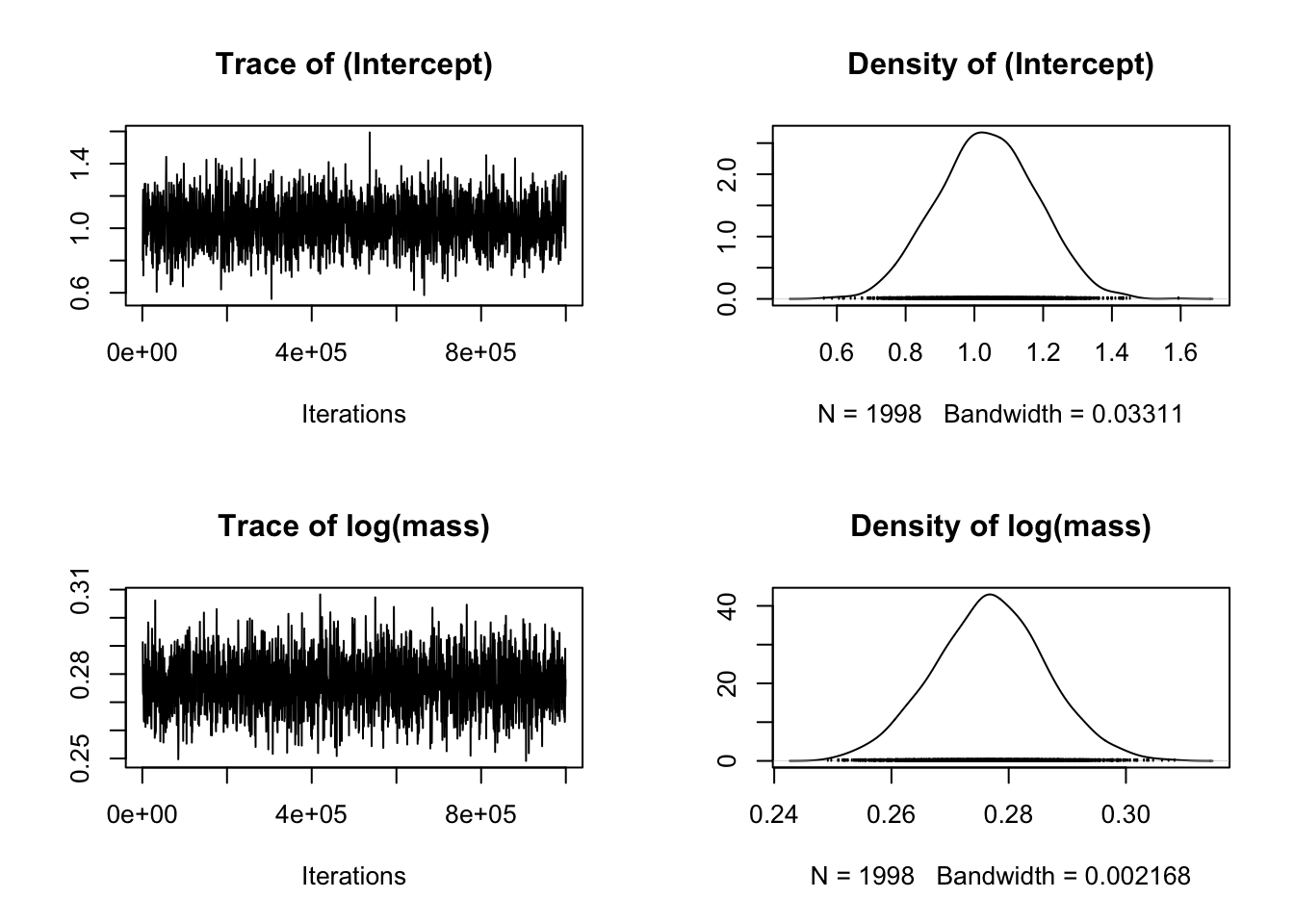
The plots on the left show a time series of the values of samples of the posterior distribution. The plots on the right show the same data as a distribution. We are looking for a “furry caterpillar” on the left hand plots, suggesting that the values are fluctuating about a largely unchanging mean value of each parameter. On the right hand plots we hope to see a distribution with one clear peak. The rows show the different parameters of the model from the fixed effects component, i.e. the intercept, the slope (labelled as log(mass)).
If it doesn’t look like the caterpillar is converging near the start of the plots that suggests you might need to increase the burnin. If there’s still a lot of fluctuation up and down you might need to increase burnin and the number of iterations. If the autocorrelation is high (see below) you might need to increase the thinning interval.
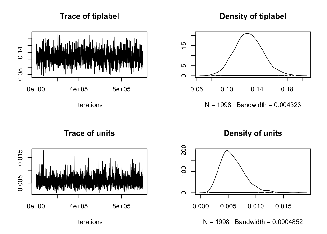 We interpret these in the same way as above except the first row is the random effect that contains the information from the phylogeny, and the second row is the residual variance. This is called units in
 MCMCglmm.
Mean centring and scaling your variables to unit
variance. Often people advise that you rescale numeric
variables so they are mean centred and scaled to unit variance. This can
be really helpful if you’ve got models with multiple numeric variables
that are quite different in scale (i.e. one ranges from 1 to 3 and one
from 100 to 1000). If your models are not converging this may also help.
To do this in R using functions from the tidyverse
package:
mydata <- mydata %>% mutate(variable1_Z = scale(log(mydata\(variable1))) %>% mutate(variable2_Z = scale(abs(mydata\)variable2)))
Just remember to reverse the transformation when trying to interpret any parameter estimates on the scale of the original variable.
These plots look fine to me! :). Remember because of the nature of MCMC we won’t have the exact same plots here, don’t worry!
We can also calculate the effective sample size (ESS) as follows.
## [1] 1998This is above 200 so the model has converged.
We should also check the validity of the posterior by looking at levels of autocorrelation…
## , , tiplabel
##
##              tiplabel        units
## Lag 0      1.00000000 -0.526793220
## Lag 500   -0.01961702  0.001163258
## Lag 2500   0.02760427 -0.013775871
## Lag 5000  -0.02899116  0.006129946
## Lag 25000 -0.01119349 -0.006134928
##
## , , units
##
##                tiplabel        units
## Lag 0     -0.5267932199  1.000000000
## Lag 500   -0.0006145319 -0.003037141
## Lag 2500  -0.0187737699 -0.016918298
## Lag 5000   0.0064124393 -0.015999863
## Lag 25000 -0.0173105728  0.015958313
Ideally, all samples of the posterior distribution should be independent, and the autocorrelation for all lag values greater than zero should be near zero. These values look OK - they’re mostly below 0.03 which is pretty close to zero - but we could try and improve them by increasing the thinning interval and the number of iterations if we needed to.
7.8 MCMC outputs
Now we can finally look at the results using summary.
##             post.mean  l-95% CI  u-95% CI eff.samp        pMCMC
## (Intercept) 1.0375044 0.7484659 1.2955290 1998.000 0.0005005005
## log(mass)   0.2768096 0.2581998 0.2955905 3277.781 0.0005005005
This gives us a similar output to the other models we’ve used previously, except the numbers come from the posterior distribution. We get the mean value of the intercept from the posterior, its 95% credible interval (the Bayesian equivalent of confidence intervals), its effective sample size, and an associated p value testing whether the value is signficantly different from zero. The second row shows the same information for the slope (log(mass)).
Here neither of the posterior distributions for the intercept or slope overlaps zero, so we can consider them both statistically supported. In a paper/report/thesis we’d report these parameter estimates and their credible intervals. I’d rarely report the MCMCp values. p values don’t really belong in a Bayesian world.
Remember we also need to look at results for the random effect variances. Generally the mode of the posterior is a better thing to look at here than the mean of the posterior, as the mode tells us where the peak of the posterior is. We can look at these using posterior.mode. Recall that units is what MCMCglmm calls the residual variance.
##   tiplabel      units
## 0.11949510 0.00491087
We also need the 95% credible intervals for these components:
##                lower      upper
## tiplabel 0.095286046 0.16795035
## units    0.002140634 0.01023753
## attr(,"Probability")
## [1] 0.9499499
While testing the significance of fixed effects by evaluating whether or not their posterior distributions overlap zero is simple and valid, this approach does not work for variance components. Variance components should be positive so even when a random effect is not meaningful, the posterior distribution will never overlap zero.
If we really care about whether a random effect is “significant”, we can fit a model without the random effect, and a model with the random effect, and then compare them using DIC (smaller DIC = better model). To get the DIC of the model we just do:
## [1] -354.1069If the model with the random effect has the lowest DIC, we can say that inclusion of the term statistically justifiable. DIC has a lot of issues however, and this won’t be appropriate in all cases. Luckily in the case of our phylogenetic random effect we already have a very good reason for including it in the model, whether or not it is “significant”. We can also look at \(\lambda\) to assess the amount of phylogenetic signal in the model. This should give us a good idea of occasions where adding the phylogenetic random effect is not appropriate.
7.9 Extracting lambda for MCMCglmm models
We can estimate the posterior probability of the phylogenetic signal \(\lambda\) as follows.
# Get lambda
lambda <- model_mcmcglmm$VCV[,'tiplabel']/
          (model_mcmcglmm$VCV[,'tiplabel'] + model_mcmcglmm$VCV[,'units'])
We can then get the mean and mode (for Bayesian analyses the mode is often a better measure of central tendency than the mean as it tells us where the peak of the posterior distribution is) of the posterior distribution for \(\lambda\), along with its 95% credible interval:
## [1] 0.9551432## var1
## 0.9658262## lower upper
## var1 0.9146033 0.9884231
## attr(,"Probability")
## [1] 0.9499499We could also quickly plot the whole posterior, with the mode and 95% credible intervals.
# Plot the posterior
ggplot(as.data.frame(lambda), aes(x = lambda))+
  geom_density() +
  geom_vline(xintercept = posterior.mode(lambda), colour = "red") +
  geom_vline(xintercept = HPDinterval(lambda)[[1]],
             linetype = "dotted", colour = "red") +
  geom_vline(xintercept = HPDinterval(lambda)[[2]],
             linetype = "dotted", colour = "red") +
  theme_bw()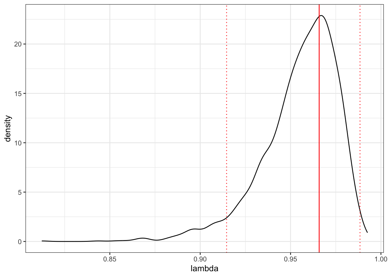
Note that this isn’t precisely \(\lambda\) as formulated by Pagel. It’s the proportion of the variance components (G + R) compromised by the phylogenetic variance component (G). But we can interpret it in the same way, i.e. 0 = no phylogenetic signal, 1 = expectation under Brownian motion.
The MCMCglmm results are very close to what we got from PGLS where intercept = 1.03, slope = 0.277, and lambda was 0.976 (95% CI: 0.924 - 1).
7.10 Checking the effects of priors
You shouldn’t stop here! It’s important to repeat the analysis with different priors to see if that would influence your conclusions. Generally I’d increase the value for nu, maybe to 1 and see what happens.
# Set up new priors for MCMCglmm
# Inverse Wishart with V = 1 and nu = 1
prior <- list(G = list(G1 = list(V = 1, nu = 1)),
              R = list(V = 1, nu = 1))

# Run the model
model_mcmcglmm2 <- MCMCglmm(log(eyesize) ~ log(mass),
                   data = mydata,
                   random = ~ tiplabel,
                   ginverse = list(tiplabel = inv.phylo),
                   prior = prior,
                   nitt = nitt, thin = thin, burnin = burnin,
                   verbose = FALSE)

# Save the model
saveRDS(model_mcmcglmm2, file = "data/model_mcmcglmm_output2.rda")
Again this takes ages to run (at least an hour on my machine), so to save you some time here I’ve run the model myself and saved it using saveRDS. You do not need to run the code above if you don’t have an hour to spare!. We can then read it back in using:
# Read in the saved model output run in advance to save time
model_mcmcglmm2 <- readRDS("data/model_mcmcglmm_output2.rda")
Let’s look at the results:
##             post.mean  l-95% CI  u-95% CI eff.samp        pMCMC
## (Intercept) 1.0317751 0.7789332 1.2671116 2097.988 0.0005005005
## log(mass) 0.2733169 0.2518094 0.2962124 1998.000 0.0005005005## tiplabel units
## 0.09779188 0.02390362## lower upper
## tiplabel 0.06703434 0.12782712
## units 0.01708881 0.03047269
## attr(,"Probability")
## [1] 0.9499499There’s no major change. Phew! We can therefore say that the difference in the priors has little effect on the outcome of the analysis (this is usual for an analysis where lots of data are available relative to the complexity of the model, but it is important to check!).
Hopefully you now see why these models are complicated and should be considered very carefully before using them. You should never skip the checking and tinkering steps.
7.11 An example using a PGLMM
A reminder. Before jumping in to these models it is vital that you have a good understanding of generalised linear models (GLMs), and generalised linear mixed models (GLMMs) including how to fit and interpret the outputs of these models in R. This is beyond the scope of this book. If you feel uncomfortable with these we suggest you go back and learn these methods first.
The example above is technically only a LMM (linear mixed model) as we used a model with Gaussian or Normal errors. But what if our response is a count? Or a proportion? We can then use the GLMM architecture of MCMCglmm to help.
For Poisson models (used generally when the response variable is a count) we actually only need to change one thing, we need to add family = "poisson" to tell MCMCglmm to fit this model. This is the same as in standard glm analyses in R. Make sure you understand GLMs before attempting PGLMMs!
For a fake example here, if we had a variable called number_of_eggs that contained count data, we could fit a model like this:
model_eggs <- MCMCglmm(number_of_eggs ~ log(mass),
                   data = mydata, family = "poisson",
                   random = ~ Species,
                   ginverse = list(Species = inv.phylo),
                   prior = prior,
                   nitt = nitt, thin = thin, burnin = burnin,
                   verbose = FALSE)
Other than these changes, everything runs as above including the priors and all the model diagnostics and checking.
If we had proportion data instead, for example the number of individuals with blue eyes and the number with red eyes, we could use a binomial model. Again this works just like in a basic glm model. Again, make sure you understand GLMs before attempting PGLMMs!
We tell R we want to use a binomial error structure using family = "binomial", and we include successes (number of frogs with red eyes) and failures (number of frogs with blue eyes) as one variable as the response using cbind to stick them together. If you’re not sure why we would do this, go back and read up on GLMs.
# Fit MCMCglmm
model_eyes <- MCMCglmm(cbind(numberred, numberblue) ~ log(mass),
                   data = mydata, family = "binomial",
                   random = ~ Species,
                   ginverse = list(Species = inv.phylo),
                   prior = prior,
                   nitt = nitt, thin = thin, burnin = burnin,
                   verbose = FALSE)
Again, other than these changes, everything runs as above including the priors and all the model diagnostics and checking. Remember the parameter estimates for binomial GLMs are log odds ratios, so might look a little strange. Again, go back and read up on GLMs if this is all sounding unfamiliar to you.
If you’re worried about whether you’ve fitted the right model, and
the additional Bayesian components of MCMCglmm are causing
you confusion, it’s fine to fit the model using a standard GLM (using
the glm function in R) to see if the results are similar.
Remember that we expect the results to be somewhat different because
glm does not incorporate the phylogeny.
7.12 Adding extra fixed and random effects
I won’t run these models here; this is just to give you an indication of how we can add complexity to these models.
Adding fixed effects to models is easy, we just add variables as we would in any other model in R. For example, if we wanted to fit this model from the PGLS exercise:
model.pgls2 <- pgls(log(eyesize) ~ log(mass) * as.factor(Adult_habitat),
                   data = frog, lambda = "ML")
We could fit a MCMCglmm model like this:
model_multiple<- model_mcmcglmm <- MCMCglmm(log(eyesize) ~ log(mass) *
                                         as.factor(Adult_habitat),
                   data = mydata,
                   random = ~ Species,
                   ginverse = list(Species = inv.phylo),
                   prior = prior,
                   nitt = nitt, thin = thin, burnin = burnin)
Note that we are adding fixed effects in this example. If we want to add more random effects we need to be a bit more careful because we need to remember to define the priors for those random effects too.
Let’s say we wanted to fit a model with phylogeny as a random effect and a random effect of Sex. We’d now have two random effects in the G-structure.
We would define the priors as follows. Note that Sex is referred to as G2.
prior2 <- list(G = list(G1 = list(V = 1, n = 0.002),
               G2 = list(V = 1, n = 0.002)),
               R = list(V = 1, n = 0.002))
We’d then fit the model as follows.
model_new <- model_mcmcglmm <- MCMCglmm(log(eyesize) ~ log(mass),
                   data = mydata,
                   random = ~ Species + Sex,
                   ginverse = list(Species = inv.phylo),
                   prior = prior2,
                   nitt = nitt, thin = thin, burnin = burnin)
Note that this gets more complex if you want to fit hierarchical or repeated measures type models so we recommend reading the materials below, and getting a thorough understanding of mixed models, before attempting this.
7.13 Summary
You should now know how to perform a GLMM analysis in R using the package MCMCglmm.
I also recommend reading the following if you want to know more: https://math.umd.edu/~slud/s770/LecSlides/Lecs19to26/CourseNotesMCMCglmm.pdf
7.14 Practical exercises
In the data folder there is another tree (primate-tree.nex) and dataset (primate-data.csv) for investigating the evolution of primate life-history variables. These data come from the PanTHERIA database [26] and 10kTrees [27].
Let’s repeat the analyses we did in the PGLS chapter but using MCMCglmm. We will investigate the relationship between gestation length in Primates and their body size.
Read in the tree and data, then prepare them for a PCM analysis (you may have already done this in a previous exercise which should save you some time). Fit a MCMCglmm model to investigate the relationship between log gestation length (y = log(GestationLen_d)) and log body size (x = log(AdultBodyMass_g)) in Primates. Don’t forget to check that the model has converged, and to look at the model diagnostics and for autocorrelation.
Then answer the following questions.
What is \(\lambda\) in the model?
What are the 95% credible intervals (HPD) around \(\lambda\)?
Plot the \(\lambda\) profile for the the maximum likelihood estimate of \(\lambda\).
Is there a significant relationship between log gestation length and log body size? What is the slope of this relationship?