Chapter 5 Phylogenetic Signal in R
Phylogenetic signal is the pattern where close relatives have more similar trait values than more distant relatives. The aims of this exercise are to learn how to use R to estimate phylogenetic signal using Pagel’s \(\lambda\) Pagel (1999) and Blomberg’s K (Blomberg, Garland Jr, and Ives 2003).
We will be using the evolution of eye size in frogs as an example. The data and modified tree come from K. N. Thomas et al. (2020), and the original tree comes from Feng et al. (2017). I’ve removed a few species and a few variables to make things a bit more straightforward. If you want to see the full results check out K. N. Thomas et al. (2020)!
Before you start
- Open the
05-PhyloSignal.RProjfile in the05-PhyloSignalfolder to open your R Project for this exercise.
You will also need to install the following packages:
tidyverse- for reading, manipulating and plotting dataape- functions for reading, plotting and manipulating phylogeniesgeiger- to check species in the tree and data matchphytools- to estimate \(lambda\) and Kcaper- to estimate D
5.1 Preparation
To begin we need to load the packages for this practical.
# Load the packages
library(tidyverse)
library(ape)
library(geiger)
library(phytools)
library(caper)
Next we need to prepare the tree and data for the analyses. In the 04-Preparation exercise we read in our tree and data, checked them, and matched them so only species in both were retained. Please refer to that exercise for more details on how and why we do these things, or run through it now if you haven’t previously.
It is important to do these things before beginning a phylogenetic comparative analysis, so let’s run through that code again here.
# Read in the data
frogdata <- read_csv("data/frog-eyes.csv")
# Check everything loaded corrected
glimpse(frogdata)
## Rows: 215
## Columns: 11
## $ Binomial <chr> "Allophryne_ruthveni", "Eupsophus_roseus", "Alytes_obstetricans", "…
## $ Family <chr> "Allophrynidae", "Alsodidae", "Alytidae", "Alytidae", "Aromobatidae…
## $ Genus <chr> "Allophryne", "Eupsophus", "Alytes", "Discoglossus", "Allobates", "…
## $ tiplabel <chr> "Allophryne_ruthveni_Allophrynidae", "Eupsophus_roseus_Alsodidae", …
## $ Adult_habitat <chr> "Scansorial", "Ground-dwelling", "Ground-dwelling", "Ground-dwellin…
## $ Life_history <chr> "Free-living larvae", "Free-living larvae", "Free-living larvae", "…
## $ Sex_dichromatism <chr> "Absent", "Absent", "Absent", "Absent", "Absent", "Absent", "Absent…
## $ SVL <dbl> 23.76667, 38.37500, 37.46667, 62.64000, 25.60000, 27.03333, 38.4000…
## $ mass <dbl> 1.0000000, 7.5000000, 6.6666667, 24.4000000, 2.1000000, 2.4666667, …
## $ rootmass <dbl> 0.9917748, 1.9273451, 1.8690601, 2.8885465, 1.2549697, 1.3507613, 1…
## $ eyesize <dbl> 3.200000, 5.362500, 6.366667, 7.550000, 4.116667, 3.783333, 4.75000…To load the tree we will use read.nexus.
# Read in the tree
frogtree <- read.nexus("data/frog-tree.nex")
# Check it loaded correctly
str(frogtree)
## List of 4
## $ edge : int [1:426, 1:2] 215 216 217 218 219 220 221 222 223 224 ...
## $ edge.length: num [1:426] 0.166 0.114 0.102 0.4 0.133 ...
## $ Nnode : int 213
## $ tip.label : chr [1:214] "Ascaphus_truei_Ascaphidae" "Leiopelma_hochstetteri_Leiopelmatidae" "Alytes_obstetricans_Alytidae" "Discoglossus_pictus_Alytidae" ...
## - attr(*, "class")= chr "phylo"
## - attr(*, "order")= chr "cladewise"Remember to check the tree is dichotomous, i.e. has no polytomies, rooted, and ultrametric.
# Check whether the tree is binary
# We want this to be TRUE
is.binary(frogtree)
## [1] TRUE# Check whether the tree is rooted
# We want this to be TRUE
is.rooted(frogtree)## [1] TRUE# Check whether the tree is ultrametric
# We want this to be TRUE
is.ultrametric(frogtree)## [1] TRUENext check that the species names match up in the tree and the data. This should reveal any typos and/or taxonomic differences that need to be fixed before going any further.
# Check whether the names match in the data and the tree
check <- name.check(phy = frogtree, data = frogdata,
                    data.names = frogdata$tiplabel)
# Look at check
check
## $tree_not_data
## [1] "Incilius_nebulifer_Bufonidae" "Leptobrachella_bidoupensis_Megophryidae"
## [3] "Microhyla_fissipes_Microhylidae" "Microhyla_marmorata_Microhylidae"
##
## $data_not_tree
## [1] "Gastrophryne_carolinensis_Microhylidae" "Leptobrachella_dringi_Megophryidae"
## [3] "Megophrys_gerti_Megophryidae" "Microhyla_pulverata_Microhylidae"
## [5] "Oreobates_quixensis_Strabomantidae"Here all the excluded species are excluded because they are genuinely missing, not because of any typos, so we can move on.
Next we exclude species that are not in both the tree and the data, using the following code:
# Remove species missing from the data
mytree <- drop.tip(frogtree, check$tree_not_data)

# Remove species missing from the tree
matches <- match(frogdata$tiplabel, check$data_not_tree, nomatch = 0)
mydata <- subset(frogdata, matches == 0)
Finally we check the tree and data have the same number of species:
# Look at the tree summary
str(mytree)
## List of 4
## $ edge : int [1:418, 1:2] 211 212 213 214 215 216 217 218 219 220 ...
## $ edge.length: num [1:418] 0.166 0.114 0.102 0.4 0.133 ...
## $ Nnode : int 209
## $ tip.label : chr [1:210] "Ascaphus_truei_Ascaphidae" "Leiopelma_hochstetteri_Leiopelmatidae" "Alytes_obstetricans_Alytidae" "Discoglossus_pictus_Alytidae" ...
## - attr(*, "class")= chr "phylo"
## - attr(*, "order")= chr "cladewise"# Look at the data
glimpse(mydata)## Rows: 210
## Columns: 11
## $ Binomial <chr> "Allophryne_ruthveni", "Eupsophus_roseus", "Alytes_obstetricans", "…
## $ Family <chr> "Allophrynidae", "Alsodidae", "Alytidae", "Alytidae", "Aromobatidae…
## $ Genus <chr> "Allophryne", "Eupsophus", "Alytes", "Discoglossus", "Allobates", "…
## $ tiplabel <chr> "Allophryne_ruthveni_Allophrynidae", "Eupsophus_roseus_Alsodidae", …
## $ Adult_habitat <chr> "Scansorial", "Ground-dwelling", "Ground-dwelling", "Ground-dwellin…
## $ Life_history <chr> "Free-living larvae", "Free-living larvae", "Free-living larvae", "…
## $ Sex_dichromatism <chr> "Absent", "Absent", "Absent", "Absent", "Absent", "Absent", "Absent…
## $ SVL <dbl> 23.76667, 38.37500, 37.46667, 62.64000, 25.60000, 27.03333, 38.4000…
## $ mass <dbl> 1.0000000, 7.5000000, 6.6666667, 24.4000000, 2.1000000, 2.4666667, …
## $ rootmass <dbl> 0.9917748, 1.9273451, 1.8690601, 2.8885465, 1.2549697, 1.3507613, 1…
## $ eyesize <dbl> 3.200000, 5.362500, 6.366667, 7.550000, 4.116667, 3.783333, 4.75000…Don’t forget to ensure the data are a data frame:
# Convert to a dataframe
mydata <- as.data.frame(mydata)
# Check this is now a data frame
class(mydata)
## [1] "data.frame"Now we’re ready to run our analyses!
5.2 Estimating phylogenetic signal for continuous variables
As is common in R, there are a number of ways to estimate Pagel’s \(\lambda\) and Blomberg’s K. I’ve chosen to show you the way implemented in the package phytools because it allows you to use the same function for both.
Why do we look at two different measures of phylogenetic signal? We don’t have to, you could choose one and stick to it. However, I guarantee if you choose one then a reviewer/your supervisor/boss will ask for the other, so why not do both and pop one in the appendix?
Let’s estimate \(\lambda\) for log eye size.
The first thing we need to do is to create an object in R that only contains the variable required, and the species names (so we can match it up to the tree).
We can use the function pull to extract just the eye size values, and we can log transform all these numbers using log if we want to work with log eye size values.
# Create logEye containing just log eye size length values
logEye <- log(pull(mydata, eyesize))
# Look at the first few rows
head(logEye)
## [1] 1.163151 1.679430 1.851076 2.021548 1.415044 1.330605Notice that this is currently just a long list of numbers. We can then name these values with the species names from mydata using the function names. Note that this requires the trait data is in the same order as the tree tip labels, but luckily make.treedata does this automatically.
# Give log Eye names = species names at the tips of the phylogeny
names(logEye) <- mydata$tiplabel
# Look at the first few rows
head(logEye)
## Allophryne_ruthveni_Allophrynidae Eupsophus_roseus_Alsodidae
## 1.163151 1.679430
## Alytes_obstetricans_Alytidae Discoglossus_pictus_Alytidae
## 1.851076 2.021548
## Allobates_femoralis_Dendrobatidae Arthroleptis_poecilonotus_Arthroleptidae
## 1.415044 1.330605Now we have a list of values with associated species names.
5.2.1 Pagel’s \(\lambda\)
We can now estimate \(\lambda\) using the function phylosig:
lambdaEye <- phylosig(mytree, logEye, method = "lambda", test = TRUE)test = TRUE specifies that we want to run a likelihood ratio test to determine if \(\lambda\) is significantly different from 0.
To look at the output we just type in the name of the model; lambdaEye in this case
lambdaEye##
## Phylogenetic signal lambda : 0.802864
## logL(lambda) : -112.137
## LR(lambda=0) : 62.803
## P-value (based on LR test) : 2.28447e-15The \(\lambda\) estimate for log eye size is around 0.803. logL is the log-likelihood, LR(lambda=0) is the log-likelihood for \(\lambda\) of 0, and P-value is the p value from a likelihood ratio test testing whether \(\lambda\) is significantly different from 0 (no phylogenetic signal).
Here P < 0.001. We interpret this as \(\lambda\) being significantly different from 0, i.e. there is significant phylogenetic signal in log eye size.
5.2.2 Blomberg’s K (Blomberg et al 2003)
To estimate Blomberg’s K we also use phylosig but with method = K.
KEye <- phylosig(mytree, logEye, method = "K", test = TRUE, nsim = 1000)Additionally we add the argument nsim = 1000. This is because we need to use a randomisation test to determine whether K is significantly different from 0. phylosig randomly assigns the trait values to the species and then calculates K as many times as we ask it to in nsim (number of simulations). Here we asked for 1000. After the random simulations are run, the observed value of K is then compared to the randomized values. The p value tells us how many times out of 1000, a randomised value of K is more extreme than the observed value. If this number is low, the p value is low (e.g. if 5 out of 1000 randomised values of K are more extreme than the observed value p = 5/1000 = 0.005).
As above, to look at the output we just type in the name of the model; KEye in this case
KEye##
## Phylogenetic signal K : 0.283009
## P-value (based on 1000 randomizations) : 0.001K for log eye size is 0.283. The p value tells us how many times out of 1000, a randomised value of K is more extreme than the observed value. If this number is low, the p value is low (e.g. if 5 out of 1000 randomised values of K are more extreme than the observed value p = 5/1000 = 0.005). Here p = 0.001, suggesting that only 1 randomised value of K was more extreme than the observed value.
We interpret this as K being significantly different from 0, i.e. there is significant phylogenetic signal in log eye size.
Remember that when fitting models to account for phylogenetic non-independence, it is not phylogenetic signal in the individual variables that is important. It is phylogenetic signal in the residuals of the model that matters. Evidence of phylogenetic signal in variable X (or variable Y) does not necessarily mean that there will be phylogenetic signal in the residuals of a model correlating variable X with variable Y. Conversely, lack of evidence of phylogenetic signal in variable X (or variable Y) does not necessarily mean that there will be no phylogenetic signal in the residuals of a model correlating variable X with variable Y.
5.3 Estimating phylogenetic signal for non-continuous variables
Not all variables are continuous, some are categorical, some are binary. For example in the frog data Adult_habitat, Life_history and Sex_dichromatism are categorical variables. We can also code Sex_dichromatism as a binary variable if we code Absent as 0 and Present as 1.
glimpse(mydata)## Rows: 210
## Columns: 11
## $ Binomial <chr> "Allophryne_ruthveni", "Eupsophus_roseus", "Alytes_obstetricans", "…
## $ Family <chr> "Allophrynidae", "Alsodidae", "Alytidae", "Alytidae", "Aromobatidae…
## $ Genus <chr> "Allophryne", "Eupsophus", "Alytes", "Discoglossus", "Allobates", "…
## $ tiplabel <chr> "Allophryne_ruthveni_Allophrynidae", "Eupsophus_roseus_Alsodidae", …
## $ Adult_habitat <chr> "Scansorial", "Ground-dwelling", "Ground-dwelling", "Ground-dwellin…
## $ Life_history <chr> "Free-living larvae", "Free-living larvae", "Free-living larvae", "…
## $ Sex_dichromatism <chr> "Absent", "Absent", "Absent", "Absent", "Absent", "Absent", "Absent…
## $ SVL <dbl> 23.76667, 38.37500, 37.46667, 62.64000, 25.60000, 27.03333, 38.4000…
## $ mass <dbl> 1.0000000, 7.5000000, 6.6666667, 24.4000000, 2.1000000, 2.4666667, …
## $ rootmass <dbl> 0.9917748, 1.9273451, 1.8690601, 2.8885465, 1.2549697, 1.3507613, 1…
## $ eyesize <dbl> 3.200000, 5.362500, 6.366667, 7.550000, 4.116667, 3.783333, 4.75000…Estimating phylogenetic signal in categorical variables is tricky. Let’s take Adult_habitat as an example. In this variable we have the following categories:
mydata %>%
 dplyr::select(Adult_habitat) %>%
 distinct()
## Adult_habitat
## 1 Scansorial
## 2 Ground-dwelling
## 3 Subfossorial
## 4 Semiaquatic
## 5 Aquatic
## 6 FossorialRemember with phylogenetic signal we are looking for the pattern where close relatives are more similar to one another than more distant relatives. For these categories, it would be sensible to say we had high phylogenetic signal if, for example, all toads are Semiaquatic, and all tree frogs are Scansorial (climbers). But what if some toads are Semiaquatic but others are Ground-dwelling? If we don’t know how species transition from state to state, it’s hard to know what we might expect to see as evolutionary distance between species increases. We might sensibly assume that species easily evolve from Semiaquatic to Aquatic, or from Subfossorial to Fossorial (burrowing), but what about changes from Aquatic to Fossorial? All of this makes phylogenetic signal for categorical variables a bit of a mess.
There are a couple of, more or less satisfying, solutions…
Do we actually need to know the phylogenetic signal for these variables? For the models we are interested in phylogenetic signal in the residuals, so maybe we don’t care about phylogenetic signal in the variables? Unless there is a real need, don’t bother! You could visualise what is going on instead by adding colours to the tips of the phylogeny to represent the different categories. This should give you an idea about whether categories cluster in different clades or not.
We could code our categories numerically then use \(\lambda\) and K as usual. This is only suitable if the categories are ordered, and if the difference between each pair of categories can be considered equal. For example, a variable that has low, medium and high values could be coded as low = 1, medium = 2, and high = 3. Again this is not ideal, but will give you an answer. I’d avoid this if possible.
We could recode these as binary variables and use D (Fritz and Purvis 2010). For example, creating a new variable called Aquatic, and coding each species as 0 = not aquatic; 1 = aquatic. This is probably the best solution.
5.3.1 D
We can estimate D using the function phylo.d in the caper package.
First we’d need to set up a binary (0,1) variable. Let’s look at Sex_dichromatism as this only has two categories already (Absent and Present).
mydata %>%
  group_by(Sex_dichromatism) %>%
  summarise(n())
## # A tibble: 3 × 2
## Sex_dichromatism `n()`
## <chr> <int>
## 1 Absent 150
## 2 Present 24
## 3 <NA> 36There are 36 species without data for this variable. If we were doing something like PGLS (see next exercise), caper would be fine with this, but for phylo.d we can only work with data without NAs. To fix this, we can use filter to exclude the species with NAs, but we will also need to remove these species from the tree.
Let’s first go back to mydata so we can exclude the species without Sex_dichromatism data, making frogdata2.
# Filter out species with no Sex_dichromatism data
mydata2 <-
  mydata %>%
  filter(!is.na(Sex_dichromatism))
Next we need to check the matching species in the tree and the new dataset and remove the missing species from the tree:
# Check whether the names match in the data and the tree
check2 <- name.check(phy = mytree, data = mydata2,
                    data.names = mydata2$tiplabel)
# Remove species missing from the data
mytree2 <- drop.tip(mytree, check2$tree_not_data)
Now we can go back to our workflow, but using mydata2 and mytree2.
We also need the variable Sex_dichromatism to be either 0 or 1. We can do this fairly easily using mutate to create a new variable called sex_di_binary.
mydata2 <-
  mydata2 %>%
  # Make a new variable called sex_di_binary
  # which is Sex_dichromatism expressed as numbers
  # i.e. Absent = 1 and Present = 2.
  # To make these 0 and 1 instead we just use -1
  mutate(sex_di_binary = as.numeric(as.factor(Sex_dichromatism)) - 1)
To use phylo.d we need the caper package. caper requires you to first combine the phylogeny and data into one object using the function comparative.data.
Note that vcv = TRUE stores a variance covariance matrix of your tree (you will need this for the pgls function in the next exercise). na.omit = FALSE stops the function from removing species without data for all variables. warn.dropped = TRUE will tell you if any species are not in both the tree and the data and are therefore dropped from the comparative data object. We need to use as.data.frame before data2 as using the tidyverse functions above to change the sexual dimorphism scores has made it a combined data frame and tibble (a special kind of data frame for the tidyverse) but comparative.data only wants the data frame.
frog <- comparative.data(phy = mytree2, data = as.data.frame(mydata2),
                            names.col = tiplabel, vcv = TRUE,
                            na.omit = FALSE, warn.dropped = TRUE)
This function will give a warning telling you that some species have been dropped. Always make sure you check the list of dropped species is what you expected, as it often reveals typos in your species names, or mismatches in taxonomies used etc.
You can view the dropped species using:
frog$dropped$unmatched.rows## character(0)This shows nothing because we already fixed the data so that all the species in the data are in the tree.
frog$dropped$tips## character(0)This also shows nothing because we already fixed the tree so that all the species in the tree are in the data.
One last bit of prep required is that D cannot be estimated where trees have zero length branches. In 04-Preparation you may recall that we dealt with polytomies by replacing them with zero length branches using the ape function mutli2di. To remove the zero length branches we are going to use the opposite function: di2multi. This deletes all zero length branches and collapses them back into polytomies.
frog$phy <- di2multi(frog$phy)Now we are ready to to estimate D.
# Estimate D
Dsexdi <- phylo.d(data = frog, names.col = tiplabel, binvar = sex_di_binary,
                  permut = 1000)

# Look at the output
Dsexdi
##
## Calculation of D statistic for the phylogenetic structure of a binary variable
##
## Data : as.data.frame(mydata2)
## Binary variable : sex_di_binary
## Counts of states: 0 = 150
## 1 = 24
## Phylogeny : mytree2
## Number of permutations : 1000
##
## Estimated D : 0.8556752
## Probability of E(D) resulting from no (random) phylogenetic structure : 0.153
## Probability of E(D) resulting from Brownian phylogenetic structure : 0.004phylo.d estimates the D value, then tests the estimated D value for significant departure from random association and a Brownian evolution threshold model (see Primer and Fritz and Purvis (2010) for more details).
Here D for Sex_dichromatism is 0.856. This is significantly different from the expectation under a Brownian threshold model (p = 0.004) but not significantly different from the trait being randomly assorted on the phylogeny (p = 0.153). So here we can say there is no significant phylogenetic signal in the trait.
We can make a really quick plot to check we agree with that statement (never take the results of any analysis at face value). It doesn’t seem like sexual dichromatism (red text) is a trait that is particularly clustered within certain taxonomic groups, so seems that D is giving us a sensible answer.
mycolours <- c("black", "red")

plot(frog$phy, show.tip.label = TRUE, tip.color =
       mycolours[as.numeric(mydata2$sex_di_binary)+1],
       no.margin = TRUE, cex = 0.4)
# Add a legend
legend("bottomleft", fill = mycolours,
       legend = c("Absent", "Present"),
       bty = "n")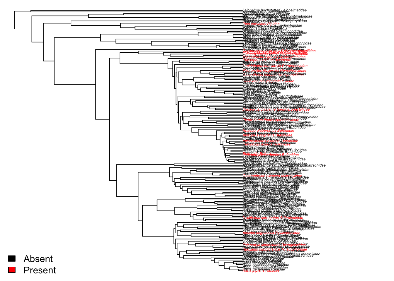
Always carefully consider what variation in values of \(\lambda\) and K and D across traits and groups really means. It may not tell you as much about your system as you think it does. Phylogenetic signal is only a pattern, not a process!
5.5 Practical exercises
In the data folder there is another tree (primate-tree.nex) and dataset (primate-data.csv) for investigating the evolution of primate life-history variables. These data come from the PanTHERIA database (Jones et al. 2009) and 10kTrees (Arnold, Matthews, and Nunn 2010).
Read in the tree and data, then prepare them for a PCM analysis (you may have already done this in the previous exercise which should save you some time). Then answer the following questions.
What is \(\lambda\) for log gestation length?
What is K for log gestation length?
What is D for social status?